Problem and Objective

For exercise 1, the Fire Department has hired me, a GIS analyst, to determine if false alarm incident data displays any clustering. The goal of this project is to perform a spatial analysis that will explain how to differentiate between real emergencies and avoid false alarms. In Exercise 2, the Fire Department has requested that determine if the value of features are clustered by performing a High/Low Clustering analysis. Exercise 3 assesses the significance of clustering on calls for service data by running a multi-distance spatial cluster analysis to determine the counts of neighboring features at several distances. Finally, in Exercise 4, the Oleander Library has requested that a spatial autocorrelation analysis be performed to determine if the data is clustered, random, or dispersed.

Analysis Procedure

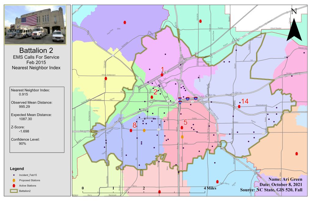
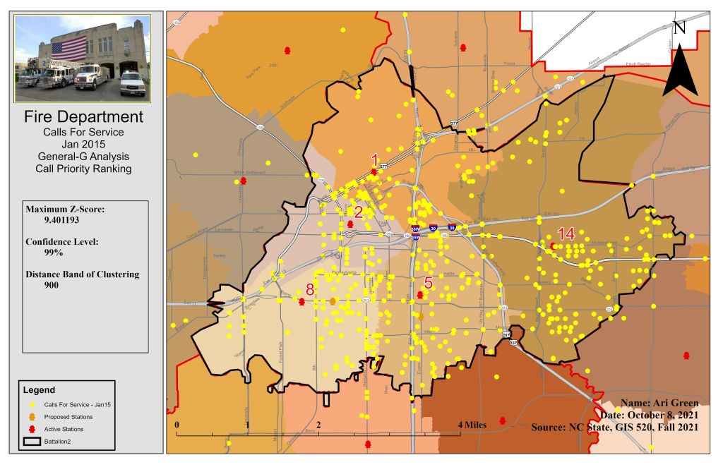
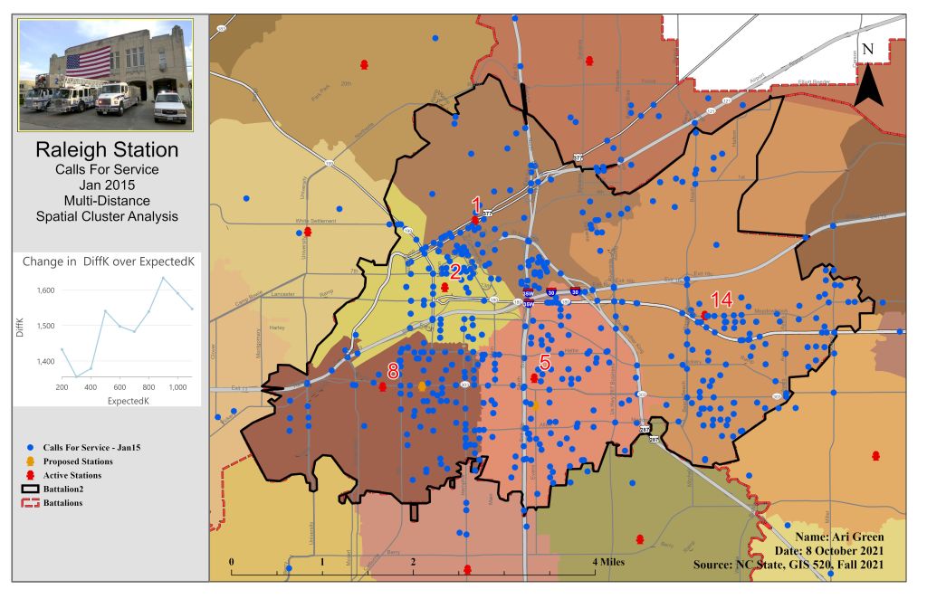
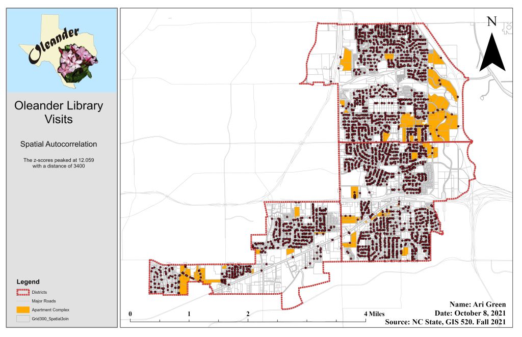
To learn how to use different geospatial statistic tools, I used ArcGIS Pro and three different types of statistical tools – descriptive, spatial, and inferential. The primary input data used for this assignment came in the form of maps that were already developed to complete tutorials (to teach) and exercises (to use fresh data on my own). This data included census data, City of Ft Worth and Oleander boundary lines, and library patron data. Geographic data can be analyzed by describing and modeling spatial distribution, patterns, processes, and spatial relationships. Spatial statistics allows me to quantify patterns and relationships I see in the data. First, I used the average nearest neighbor to determine a significant level of clustering or dispersion. The nearest neighbor ratio was 0.915 with a z-score of -1.698. This method was used to test for clustering in fire department data. The second method used was the Distance Band from Neighbor Count and High/Low Clustering tools. These tools are used to identify the clustering of values. Six different distances (700 to 1200 ft) were used to identify the peak in z-scores, which was distance 900 with a z-score of 9.401193. Next, I utilized the multi-distance spatial cluster analysis tool with the confidence envelope to measure the distance between features and determine clustering then display it in graph form. Lastly, I used the Spatial Autocorrelation tool to find clustering using attribute values and locations of features. The spatial autocorrelation tool allows me to compare the values of neighboring features by using a spatial join between point data (calls for service) and a grid (300 ft grid layer). For this tool, distances between 2800ft and 3800ft (in 200 increments) were tested. The z-score peaked the most at 3400ft at 12.059.

Results

Application and Reflection

After using several spatial statistical tools such as Average Nearest Neighbor, Distance Band from Neighbor, High/Low Clustering, multi-distance spatial cluster, and Moran’s I, I learned that these tools are essential to monitoring conditions, tracking changes over time, and comparing features. The ability to analyze clusters and distribution of data with different tools can be applied to all walks of life. For example, using the average nearest neighbor tool during the pandemic for the Spanish Flu in 1914 and Covid in 2020, could identify clusters of affected people and label it as a hotspot for spread. Another example is using the high/low clustering tool to determine higher than expected testing results from a local school’s standardized testing (to identify students who may need more help or are beyond their grade level).

Problem Description: The City of Raleigh asked its GIS analysts to identify clusters of people affected by Covid and label it as a hotspot by performing an average nearest neighbor analysis to contain the spread of Covid to one area.

Data Needed: City of Raleigh Boundary, Raleigh City Council Districts, Number of Covid Cases (tabular), and 2020 Demographic Census Data by Census Tract.

Analysis Procedures: First, analysts must use the average nearest neighbor to determine a significant level of clustering or dispersion amongst the population in the City of Raleigh. Then use the Distance Band tool to locate how close or how far the clusters are to each other to determine their value. Next, utilize the multi-distance spatial cluster analysis tool with the confidence envelope to measure the distance between population with and without covid and determine clustering. And finally, use the Spatial Autocorrelation tool to find clustering using attribute values and locations of features.